WiDS Datathon Maastricht 2021
 Anna Machens
BDSI took part in this year’s Women in Data Science datathon from Maastricht university. A Datathon is similar to a Hackathon, a weekend-long competition wheasdre you are challenged to solve problems with code. The prolems in a datathon are from different areas of Machine Learning, AI, and Data Science. The competition was part of a larger challenge hosted on kaggle.
This year’s challenge was about predicting diabetes in intensive care patients. From the Competition description:
“Getting a rapid understanding of the context of a patient’s overall health has been particularly important during the COVID-19 pandemic as healthcare workers around the world struggle with hospitals overloaded by patients in critical condition. Intensive Care Units (ICUs) often lack verified medical histories for incoming patients. A patient in distress or a patient who is brought in confused or unresponsive may not be able to provide information about chronic conditions such as heart disease, injuries, or diabetes. Medical records may take days to transfer, especially for a patient from another medical provider or system. Knowledge about chronic conditions such as diabetes can inform clinical decisions about patient care and ultimately improve patient outcomes. This year’s challenge will focus on models to determine whether a patient admitted to an ICU has been diagnosed with a particular type of diabetes, Diabetes Mellitus, using data from the first 24 hours of intensive care”
We made the first place among the participants of the Maastricht Datathon and want to share our solution here. If you want to run or experiment with the data yourself, you can try downloading the data from Kaggle. This Notebook can be downloaded here:
The path we took was the following: after a quick look at the data, we set up a tree-based gradient boosting model. We used bayesiam hyperparameter optimization to find the best hypterparameters for our model. Most of the time was then spent with feature creation and model evaluation. For completion, we will also show our steps for feature imputation and feature selection, but in the end, this did not improve the model.
import warnings
warnings.filterwarnings('ignore')

import numpy as np
import seaborn as sns
The data
The data has ~130000 entries and almost 180 columns to use as features. Each row corresponds to one patient. We want to train a model on this data to predict whether or not a patient has diabetes, given the information in the feature columns. The trained model we then apply to new data of about 10000 patients in ICU in order to estimate their probability of having diabetes.
The features can be sorted into several subgroups:
- data characterizing the patient: i.e. age, gender, ethnicity, height, weight and bmi
- data about known diseases and complications of the patient: i.e. aids, hepatic_failure, leukemia,…
- data from the first examinations, including heart-rate, blood pressure and blood tests in the first hour and on the first day. These are max and min values
- data from the [APACHE scoring system] (https://en.wikipedia.org/wiki/APACHE_II), which includes data from the first examination.
- data related to the hospital, i.e: icu_type, hospital_admit_source, elective_surgery…
import pandas as pd
df = pd.read_csv('TrainingWiDS2021.csv', index_col=0)
df_pred = pd.read_csv('UnlabeledWiDS2021.csv', index_col=0)

print('train data:', df.shape, 'test data:', df_pred.shape)
df.head()
train data: (130157, 180) test data: (10234, 179)
| encounter_id | hospital_id | age | bmi | elective_surgery | ethnicity | gender | height | hospital_admit_source | icu_admit_source | ... | h1_pao2fio2ratio_max | h1_pao2fio2ratio_min | aids | cirrhosis | hepatic_failure | immunosuppression | leukemia | lymphoma | solid_tumor_with_metastasis | diabetes_mellitus | |
|---|---|---|---|---|---|---|---|---|---|---|---|---|---|---|---|---|---|---|---|---|---|
| 1 | 214826 | 118 | 68.0 | 22.732803 | 0 | Caucasian | M | 180.3 | Floor | Floor | ... | NaN | NaN | 0 | 0 | 0 | 0 | 0 | 0 | 0 | 1 |
| 2 | 246060 | 81 | 77.0 | 27.421875 | 0 | Caucasian | F | 160.0 | Floor | Floor | ... | 51.0 | 51.0 | 0 | 0 | 0 | 0 | 0 | 0 | 0 | 1 |
| 3 | 276985 | 118 | 25.0 | 31.952749 | 0 | Caucasian | F | 172.7 | Emergency Department | Accident & Emergency | ... | NaN | NaN | 0 | 0 | 0 | 0 | 0 | 0 | 0 | 0 |
| 4 | 262220 | 118 | 81.0 | 22.635548 | 1 | Caucasian | F | 165.1 | Operating Room | Operating Room / Recovery | ... | 337.0 | 337.0 | 0 | 0 | 0 | 0 | 0 | 0 | 0 | 0 |
| 5 | 201746 | 33 | 19.0 | NaN | 0 | Caucasian | M | 188.0 | NaN | Accident & Emergency | ... | NaN | NaN | 0 | 0 | 0 | 0 | 0 | 0 | 0 | 0 |
5 rows × 180 columns
Below are the top 15 features ordered by their correlation with the target. We’ll also display the type of data (if it’s float or categorical), the fraction of missing values (between 0 and 1) and the number of unique entries. The data has many missing values. In particular, not every patient has gone through the exam and blood tests in the first hour, but also other measures have not been taken equally for all patients. We can assume that many of those are not missing at random, i.e. a doctor decided which measures to take for a patient given their situation.
# a short view of missing values and unique values in the data, as well as correlation with the target
y_df = df['diabetes_mellitus']
df = df.drop(columns=['diabetes_mellitus'])
def highlight_nas(s):
    '''
    highlight values above 0.5 in a Series yellow.
    '''
    is_max = s > 0.5
    return ['background-color: yellow' if v else '' for v in is_max]

dftypes = pd.DataFrame(df.dtypes.rename('type'))
dftypes['isnull'] = df.isnull().mean()
dftypes['unique'] = df.nunique()
dftypes['corr'] = df.corrwith(y_df)
dftypes['abs_corr'] = dftypes['corr'].apply(abs)
dftypes.sort_values(by='abs_corr', ascending=False)[['type','isnull','unique','corr']][0:15]\
        .style.apply(highlight_nas, subset=['isnull']).set_caption("Tab.1")
| type | isnull | unique | corr | |
|---|---|---|---|---|
| d1_glucose_max | float64 | 0.063331 | 538 | 0.400742 |
| glucose_apache | float64 | 0.112910 | 566 | 0.354359 |
| h1_glucose_max | float64 | 0.576788 | 612 | 0.316847 |
| h1_glucose_min | float64 | 0.576788 | 604 | 0.304520 |
| bmi | float64 | 0.034497 | 41453 | 0.169043 |
| weight | float64 | 0.026606 | 3636 | 0.155517 |
| d1_bun_max | float64 | 0.105519 | 494 | 0.146990 |
| bun_apache | float64 | 0.195233 | 476 | 0.145241 |
| d1_bun_min | float64 | 0.105519 | 471 | 0.137304 |
| d1_glucose_min | float64 | 0.063331 | 256 | 0.135848 |
| h1_bun_min | float64 | 0.806641 | 259 | 0.135157 |
| h1_bun_max | float64 | 0.806641 | 259 | 0.134985 |
| d1_creatinine_max | float64 | 0.101977 | 1247 | 0.127929 |
| d1_creatinine_min | float64 | 0.101977 | 1147 | 0.125828 |
| creatinine_apache | float64 | 0.191169 | 1198 | 0.124891 |
#uniting both train and test data for feature creation and data exploration
test_id = df_pred['encounter_id']

train_size = df.shape[0]
test_size = df_pred.shape[0]
X = pd.concat([df, df_pred], axis=0)
X = X.drop(columns=['encounter_id','hospital_id'])
X.head()
| age | bmi | elective_surgery | ethnicity | gender | height | hospital_admit_source | icu_admit_source | icu_id | icu_stay_type | ... | h1_arterial_po2_min | h1_pao2fio2ratio_max | h1_pao2fio2ratio_min | aids | cirrhosis | hepatic_failure | immunosuppression | leukemia | lymphoma | solid_tumor_with_metastasis | |
|---|---|---|---|---|---|---|---|---|---|---|---|---|---|---|---|---|---|---|---|---|---|
| 1 | 68.0 | 22.732803 | 0 | Caucasian | M | 180.3 | Floor | Floor | 92 | admit | ... | NaN | NaN | NaN | 0 | 0 | 0 | 0 | 0 | 0 | 0 |
| 2 | 77.0 | 27.421875 | 0 | Caucasian | F | 160.0 | Floor | Floor | 90 | admit | ... | 51.0 | 51.0 | 51.0 | 0 | 0 | 0 | 0 | 0 | 0 | 0 |
| 3 | 25.0 | 31.952749 | 0 | Caucasian | F | 172.7 | Emergency Department | Accident & Emergency | 93 | admit | ... | NaN | NaN | NaN | 0 | 0 | 0 | 0 | 0 | 0 | 0 |
| 4 | 81.0 | 22.635548 | 1 | Caucasian | F | 165.1 | Operating Room | Operating Room / Recovery | 92 | admit | ... | 265.0 | 337.0 | 337.0 | 0 | 0 | 0 | 0 | 0 | 0 | 0 |
| 5 | 19.0 | NaN | 0 | Caucasian | M | 188.0 | NaN | Accident & Emergency | 91 | admit | ... | NaN | NaN | NaN | 0 | 0 | 0 | 0 | 0 | 0 | 0 |
5 rows × 177 columns
Data Exploration
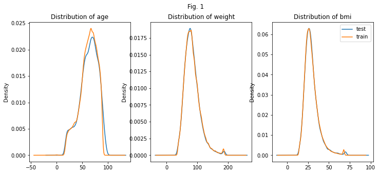
The first thing we want to understand is, whether the distributions of the features are similar for the test data and the training data. If they are, we can assume that the model performs similar on the test and training data. After checking a few features, it looks promising. No further measures are needed to adjust the distribution of the training data.
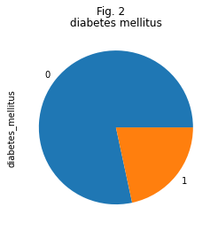
The distribution of the target variable is skewed. Many more people are healthy than diabetic.
%matplotlib inline
# comparing the distribution of train and test set for 3 features. try out other features as well.
import matplotlib.pyplot as plt


X['dataset']='train'
X['dataset'].iloc[train_size:]='test'
fig, ax = plt.subplots(1,3, figsize=(12,5))
X.groupby(['dataset'])['age'].plot.kde(title='Distribution of age', ax=ax[0])
X.groupby(['dataset'])['weight'].plot.kde(title='Distribution of weight', ax=ax[1])
X.groupby(['dataset'])['bmi'].plot.kde(title='Distribution of bmi', ax=ax[2])#, ind=50)
X.drop(columns=['dataset'],inplace=True)
plt.legend()
plt.suptitle( 'Fig. 1')
plt.show();
y_df.value_counts().plot.pie(title='diabetes mellitus')
plt.suptitle( 'Fig. 2')

plt.show();
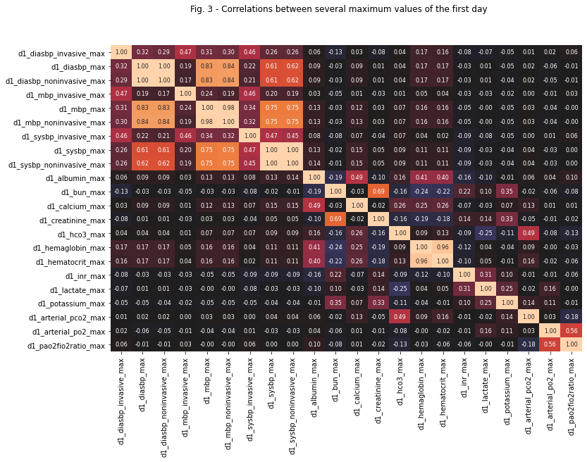
We can see how features correlate with the target in Tab.1. The blood sugar values seem to be a good predictor of diabetes, but weight or body mass index also seem very relevant. Looking at the correlation matrix of some of the blood test values with each other, we can see, that some values correlate quite strongly. Apart from all the blood pressure values in the upper left block, for which correlation is obvious, the blood urea nitrogen (bun) correlates with creatinine. Both are key indicators of renal health. And both are also among the values with comparably high correlation with the diabetes indicator. Calcium is strongly correlated with albumin as it mainly binds to this protein. Arterial pco2, the partial pressure of carbon oxide indicates how well the lungs work. It is closely related to the regulation of the bodies pH. It correlates with hco3 (bicarbonate), a byproduct of the body’s metabolism.
import gc
del (display)
# correlation of the maximum examination values for the first 24 hours. Only those with a correlation
lab_col = [c for c in X.columns if((c.startswith("h1")) | (c.startswith("d1")))]
lab_max = [col for col in lab_col if (col.endswith('max'))&(col.startswith('d1'))]
M = df[lab_max].corr()
cond = (M>0.3) | (M<-0.3)
M = M.loc[(cond).sum(axis=1)>=2,(cond).sum(axis=0)>=2]
print(M.shape)
with pd.option_context('display.max_rows', 100, 'display.max_columns', 100):
    display(M.style.background_gradient(cmap='Blues'))
(22, 22)
| d1_diasbp_invasive_max | d1_diasbp_max | d1_diasbp_noninvasive_max | d1_mbp_invasive_max | d1_mbp_max | d1_mbp_noninvasive_max | d1_sysbp_invasive_max | d1_sysbp_max | d1_sysbp_noninvasive_max | d1_albumin_max | d1_bun_max | d1_calcium_max | d1_creatinine_max | d1_hco3_max | d1_hemaglobin_max | d1_hematocrit_max | d1_inr_max | d1_lactate_max | d1_potassium_max | d1_arterial_pco2_max | d1_arterial_po2_max | d1_pao2fio2ratio_max | |
|---|---|---|---|---|---|---|---|---|---|---|---|---|---|---|---|---|---|---|---|---|---|---|
| d1_diasbp_invasive_max | 1.000000 | 0.320324 | 0.290596 | 0.474175 | 0.314042 | 0.302347 | 0.461149 | 0.263682 | 0.259751 | 0.063425 | -0.133435 | 0.031773 | -0.078941 | 0.038133 | 0.166340 | 0.155004 | -0.075539 | -0.067382 | -0.051210 | 0.005972 | 0.016085 | 0.056510 |
| d1_diasbp_max | 0.320324 | 1.000000 | 0.996682 | 0.186220 | 0.832013 | 0.841064 | 0.223667 | 0.612861 | 0.616629 | 0.090662 | -0.033129 | 0.091010 | 0.012364 | 0.043033 | 0.169462 | 0.173316 | -0.026745 | 0.006583 | -0.045627 | 0.016056 | -0.055155 | -0.010105 |
| d1_diasbp_noninvasive_max | 0.290596 | 0.996682 | 1.000000 | 0.171566 | 0.834033 | 0.843767 | 0.210190 | 0.614794 | 0.618312 | 0.091255 | -0.033029 | 0.092474 | 0.013040 | 0.041243 | 0.168346 | 0.172047 | -0.027843 | 0.009391 | -0.043272 | 0.016725 | -0.050958 | -0.006641 |
| d1_mbp_invasive_max | 0.474175 | 0.186220 | 0.171566 | 1.000000 | 0.235096 | 0.194670 | 0.456557 | 0.196863 | 0.191229 | 0.027163 | -0.054107 | 0.014021 | -0.033505 | 0.014069 | 0.051297 | 0.041084 | -0.031991 | -0.034002 | -0.020013 | 0.002967 | -0.009064 | 0.025607 |
| d1_mbp_max | 0.314042 | 0.832013 | 0.834033 | 0.235096 | 1.000000 | 0.984709 | 0.336499 | 0.745444 | 0.746367 | 0.129985 | -0.030823 | 0.124593 | 0.025816 | 0.070687 | 0.157079 | 0.160783 | -0.047253 | -0.004166 | -0.047124 | 0.029981 | -0.036830 | -0.001003 |
| d1_mbp_noninvasive_max | 0.302347 | 0.841064 | 0.843767 | 0.194670 | 0.984709 | 1.000000 | 0.321407 | 0.750361 | 0.753997 | 0.130894 | -0.029910 | 0.126792 | 0.028064 | 0.070325 | 0.158293 | 0.162325 | -0.047602 | -0.001756 | -0.047439 | 0.030932 | -0.040050 | -0.002876 |
| d1_sysbp_invasive_max | 0.461149 | 0.223667 | 0.210190 | 0.456557 | 0.336499 | 0.321407 | 1.000000 | 0.472829 | 0.450320 | 0.084315 | -0.079631 | 0.067742 | -0.035024 | 0.071140 | 0.041051 | 0.020735 | -0.090965 | -0.084060 | -0.050629 | 0.002520 | 0.014700 | 0.059473 |
| d1_sysbp_max | 0.263682 | 0.612861 | 0.614794 | 0.196863 | 0.745444 | 0.750361 | 0.472829 | 1.000000 | 0.996404 | 0.134806 | -0.015392 | 0.152015 | 0.047443 | 0.086060 | 0.110778 | 0.112535 | -0.091722 | -0.030952 | -0.039285 | 0.043861 | -0.026409 | 0.004078 |
| d1_sysbp_noninvasive_max | 0.259751 | 0.616629 | 0.618312 | 0.191229 | 0.746367 | 0.753997 | 0.450320 | 0.996404 | 1.000000 | 0.135539 | -0.014230 | 0.154194 | 0.048286 | 0.086314 | 0.112243 | 0.114425 | -0.090666 | -0.030422 | -0.040409 | 0.043812 | -0.028849 | 0.002665 |
| d1_albumin_max | 0.063425 | 0.090662 | 0.091255 | 0.027163 | 0.129985 | 0.130894 | 0.084315 | 0.134806 | 0.135539 | 1.000000 | -0.193439 | 0.489287 | -0.096105 | 0.156159 | 0.407679 | 0.400403 | -0.162161 | -0.098198 | -0.009273 | 0.063587 | 0.042213 | 0.101836 |
| d1_bun_max | -0.133435 | -0.033129 | -0.033029 | -0.054107 | -0.030823 | -0.029910 | -0.079631 | -0.015392 | -0.014230 | -0.193439 | 1.000000 | -0.027046 | 0.685037 | -0.155394 | -0.240338 | -0.220341 | 0.218123 | 0.099226 | 0.345274 | -0.018497 | -0.059367 | -0.079590 |
| d1_calcium_max | 0.031773 | 0.091010 | 0.092474 | 0.014021 | 0.124593 | 0.126792 | 0.067742 | 0.152015 | 0.154194 | 0.489287 | -0.027046 | 1.000000 | -0.020694 | 0.258172 | 0.249086 | 0.264381 | -0.070057 | -0.028668 | 0.066931 | 0.126885 | 0.005665 | 0.009696 |
| d1_creatinine_max | -0.078941 | 0.012364 | 0.013040 | -0.033505 | 0.025816 | 0.028064 | -0.035024 | 0.047443 | 0.048286 | -0.096105 | 0.685037 | -0.020694 | 1.000000 | -0.156437 | -0.192583 | -0.180116 | 0.143538 | 0.137169 | 0.333443 | -0.052045 | -0.014565 | -0.019266 |
| d1_hco3_max | 0.038133 | 0.043033 | 0.041243 | 0.014069 | 0.070687 | 0.070325 | 0.071140 | 0.086060 | 0.086314 | 0.156159 | -0.155394 | 0.258172 | -0.156437 | 1.000000 | 0.086127 | 0.125667 | -0.093874 | -0.246340 | -0.110334 | 0.487917 | -0.079805 | -0.134281 |
| d1_hemaglobin_max | 0.166340 | 0.169462 | 0.168346 | 0.051297 | 0.157079 | 0.158293 | 0.041051 | 0.110778 | 0.112243 | 0.407679 | -0.240338 | 0.249086 | -0.192583 | 0.086127 | 1.000000 | 0.957684 | -0.123911 | 0.038945 | -0.038564 | 0.086453 | -0.000514 | -0.025374 |
| d1_hematocrit_max | 0.155004 | 0.173316 | 0.172047 | 0.041084 | 0.160783 | 0.162325 | 0.020735 | 0.112535 | 0.114425 | 0.400403 | -0.220341 | 0.264381 | -0.180116 | 0.125667 | 0.957684 | 1.000000 | -0.101421 | 0.050270 | -0.011952 | 0.162995 | -0.024486 | -0.061876 |
| d1_inr_max | -0.075539 | -0.026745 | -0.027843 | -0.031991 | -0.047253 | -0.047602 | -0.090965 | -0.091722 | -0.090666 | -0.162161 | 0.218123 | -0.070057 | 0.143538 | -0.093874 | -0.123911 | -0.101421 | 1.000000 | 0.311886 | 0.104218 | -0.005626 | -0.007607 | -0.059450 |
| d1_lactate_max | -0.067382 | 0.006583 | 0.009391 | -0.034002 | -0.004166 | -0.001756 | -0.084060 | -0.030952 | -0.030422 | -0.098198 | 0.099226 | -0.028668 | 0.137169 | -0.246340 | 0.038945 | 0.050270 | 0.311886 | 1.000000 | 0.251351 | -0.017078 | 0.162697 | -0.001158 |
| d1_potassium_max | -0.051210 | -0.045627 | -0.043272 | -0.020013 | -0.047124 | -0.047439 | -0.050629 | -0.039285 | -0.040409 | -0.009273 | 0.345274 | 0.066931 | 0.333443 | -0.110334 | -0.038564 | -0.011952 | 0.104218 | 0.251351 | 1.000000 | 0.141095 | 0.107483 | -0.005299 |
| d1_arterial_pco2_max | 0.005972 | 0.016056 | 0.016725 | 0.002967 | 0.029981 | 0.030932 | 0.002520 | 0.043861 | 0.043812 | 0.063587 | -0.018497 | 0.126885 | -0.052045 | 0.487917 | 0.086453 | 0.162995 | -0.005626 | -0.017078 | 0.141095 | 1.000000 | 0.032404 | -0.181386 |
| d1_arterial_po2_max | 0.016085 | -0.055155 | -0.050958 | -0.009064 | -0.036830 | -0.040050 | 0.014700 | -0.026409 | -0.028849 | 0.042213 | -0.059367 | 0.005665 | -0.014565 | -0.079805 | -0.000514 | -0.024486 | -0.007607 | 0.162697 | 0.107483 | 0.032404 | 1.000000 | 0.562616 |
| d1_pao2fio2ratio_max | 0.056510 | -0.010105 | -0.006641 | 0.025607 | -0.001003 | -0.002876 | 0.059473 | 0.004078 | 0.002665 | 0.101836 | -0.079590 | 0.009696 | -0.019266 | -0.134281 | -0.025374 | -0.061876 | -0.059450 | -0.001158 | -0.005299 | -0.181386 | 0.562616 | 1.000000 |
#correlation heatmap
fig, heat = plt.subplots(figsize = (12,8))

heat = sns.heatmap(M, annot=True, fmt=',.2f', center=0, cbar=False, annot_kws={'size': 8})#
plt.suptitle( 'Fig. 3 - Correlations between several maximum values of the first day');
Data Pre-processing
we will encode the categorical data. Some of the categories are only in the training set and some are only in the test set. Since here we know exactly what data will be in the test set, we can drop all categories that appear either only in the test or only in the training set, because they will not be relevant for training or predicting. If we could get different test set data at a later point, this would not be a useful thing to do. But in this scenario, it will reduce unnecessary information and help to improve model evaluation. Furthermore, we drop the ‘readmission_status’ variable, as it has the same entry everywhere, as well as hospital_id and encounter_id, as they do not appear useful for the model.
# cleaning errors in the data, by exchanging maximum and minimum values, when min is larger than max.
min_max_feats=[f[:-4] for f in df.columns if f[-4:]=='_min']
for col in min_max_feats:
    X.loc[X[f'{col}_min'] > X[f'{col}_max'], [f'{col}_min', f'{col}_max']] = X.loc[X[f'{col}_min'] > X[f'{col}_max'], [f'{col}_max', f'{col}_min']].values
# selecting categorical values
hospital_categorical = ['hospital_admit_source','icu_admit_source','icu_stay_type','icu_type','icu_id']
diseases = ['aids', 'cirrhosis','hepatic_failure', 'immunosuppression', 'leukemia','lymphoma','solid_tumor_with_metastasis']
personal_categorical = ['gender','ethnicity']
cat_features = hospital_categorical+diseases+personal_categorical
# encoding categories, but only those which are in test and training set. the rest is set to -1.
for col in cat_features:
    cats_train = set(X[col].iloc[:train_size].unique())
    cats_test = set(X[col].iloc[train_size:].unique())
    categories = cats_train.intersection(cats_test)
    categories = [k for k in categories if k==k] #nan is never equal to itself :)
    print(col, cats_train.difference(cats_test), cats_test.difference(cats_train))

    X[col] = pd.Categorical(X[col], categories=categories).reorder_categories(categories)
    X[col] = X[col].cat.codes
hospital_admit_source {'ICU', 'Observation', 'Acute Care/Floor', 'Other', 'PACU'} set()
icu_admit_source set() set()
icu_stay_type set() set()
icu_type set() set()
icu_id {636, 641, 135, 650, 907, 398, 654, 1048, 417, 677, 424, 425, 170, 426, 427, 428, 174, 302, 176, 429, 430, 431, 432, 556, 1076, 823, 312, 956, 830, 195, 970, 971, 335, 976, 338, 978, 468, 470, 471, 984, 89, 474, 552, 603, 989, 862, 479, 480, 482, 997, 230, 365, 366, 493, 494, 241, 242, 498, 1010, 634, 248, 377, 506, 252} {899, 900, 901, 269, 912, 147, 924, 544, 162, 931, 166, 934, 935, 941, 436, 443, 446, 447, 1093, 453, 1095, 456, 713, 1098, 716, 1101, 720, 465, 723, 724, 725, 726, 728, 729, 351, 101, 361, 1003}
aids set() set()
cirrhosis set() set()
hepatic_failure set() set()
immunosuppression set() set()
leukemia set() set()
lymphoma set() set()
solid_tumor_with_metastasis set() set()
gender set() set()
ethnicity set() set()
apache_cols = [col for col in X.columns if col.endswith('apache')]
d1_cols = [col for col in X.columns if col.startswith('d1_')]
base = set(col[3:-4] for col in d1_cols)
Feature imputation
we used k-nearest neighbor algorithm, to impute features. For many features, like hemaglobin values this resulted in a very high r^2. However, the high r^2 does not necessarily mean, that the true underlying feature value can be found. It is likely, that values are not missing at random. There could be a meaningful pattern in the missingness which makes good imputation very difficult if not impossible. In the end, feature imputation did not seem to change much on our final score.
# the quality of kNN imputation. Additionally to the missing values, we impute known unseen values, to measure the imputation quality by the prediction on these.
def kNN_score(knn_model, Xfit, yfit):
    """ checks how well a kNN model can predict the target in yfit given the features in Xfit
    returns: the average 3-fold cross-validation score (r^2)"""

    kfold = KFold(n_splits=3)
    avg_score=0
    for train_index, test_index in kfold.split(Xfit, yfit):
        X_train, X_test = Xfit.iloc[train_index], Xfit.iloc[test_index]
        y_train, y_test = yfit.iloc[train_index], yfit.iloc[test_index]
        knn_model.fit(X_train, y_train)
        score = knn_model.score(X_test, y_test, sample_weight=None)
        print(score,end=', ')
        avg_score+=score/3
    print('score = ', avg_score)
    return avg_score
# decision whether or not a value is imputed depends on 2 things, the quality of imputation, and how many values can be imputed with the model
def try_to_impute_target(X, target, features, min_score=0.85):
    X_k = X[features]
    y_k = X[target]
    cond = (~X_k.isnull().any(axis=1))
    cond_test = cond&(y_k.isnull())
    cond_train = cond&(~y_k.isnull())
    Xfit = X_k[cond_train]
    yfit = y_k[cond_train]
    imputable_rows = cond_test.sum()
    training_rows = cond_train.sum()
    print(target, imputable_rows, training_rows )
    if imputable_rows>100:
        knn_model = KNeighborsRegressor(n_neighbors=50)
        if kNN_score(knn_model, Xfit, yfit)>min_score:
            print('imputing', target)
            knn_model.fit(Xfit, yfit)
            X['imp_'+target] = y_k#.isnull().astype(int)
            X['imp_'+target][cond_test] = knn_model.predict(X_k[cond_test])
# we set the features on which the values we want to impute depend. These are the features that kNN uses to find the closest values.
imputers = {

'h1_bun_max':['d1_bun_max','d1_bun_min'],#,'d1_bun_mean'],#0.973
'h1_bun_min':['d1_bun_max','d1_bun_min','bun_apache','h1_bun_max'],#'d1_bun_mean',#0.993
'd1_hemaglobin_min':['d1_wbc_max','d1_wbc_min','d1_hematocrit_max','d1_hematocrit_min'],#,'d1_wbc_mean',,'d1_hematocrit_mean'0.932
'd1_hemaglobin_max':[ 'd1_wbc_max','d1_wbc_min','d1_hematocrit_max','d1_hematocrit_min','d1_hemaglobin_min'],#,'d1_wbc_mean',,'d1_hematocrit_mean'#0.942
'd1_hematocrit_min':['d1_hemaglobin_max','d1_hemaglobin_min'],#'d1_hemaglobin_mean'],#0.941
'd1_hematocrit_max':['d1_hemaglobin_max','d1_hemaglobin_min', 'd1_hematocrit_min'],#,'d1_hemaglobin_mean'0.968

'glucose_apache':['d1_glucose_max','d1_glucose_min','d1_creatinine_max','d1_albumin_max','d1_bun_max' ],#,'d1_glucose_mean',,'d1_glucose_range',0.899
'h1_hco3_min':['d1_hco3_max','d1_creatinine_max', 'd1_hco3_min' ],#'d1_hco3_mean',0.855
'h1_hco3_max':['d1_hco3_max','d1_creatinine_max', 'd1_hco3_min','h1_hco3_min' ],#'d1_hco3_mean',
'h1_creatinine_min':[ 'd1_creatinine_max', 'd1_creatinine_min', 'creatinine_apache',
                      'd1_hco3_max', 'd1_bun_max','h1_hco3_max' ],#0.848
'h1_creatinine_max':[ 'd1_creatinine_max', 'd1_creatinine_min', 'creatinine_apache',
                      'd1_hco3_max', 'd1_bun_max','h1_hco3_max' ,'h1_creatinine_min'],#0.874
'h1_arterial_ph_max':['d1_arterial_ph_max','d1_arterial_ph_min','ph_apache']#,'d1_hco3_min','d1_lactate_max''d1_arterial_pco2_max'],'paco2_for_ph_apache'
}
           #
from sklearn.model_selection import KFold
from sklearn.neighbors import KNeighborsRegressor

for target, features in imputers.items():

    try_to_impute_target(X, target, features)
h1_bun_max 98378 27171
0.9726283228112811, 0.9774464400753587, 0.9738850251826521, score =  0.9746532626897639
imputing h1_bun_max
h1_bun_min 0 25322
d1_hemaglobin_min 591 120860
0.9268327938835484, 0.9236312409596664, 0.9260098268049484, score =  0.9254912872160543
imputing d1_hemaglobin_min
d1_hemaglobin_max 0 120860
d1_hematocrit_min 240 122670
0.9403018930238896, 0.9385710076854169, 0.9299885878584262, score =  0.9362871628559108
imputing d1_hematocrit_min
d1_hematocrit_max 0 122670
glucose_apache 2543 60166
0.9076695733966385, 0.8919699035572255, 0.8964962472586244, score =  0.8987119080708295
imputing glucose_apache
h1_hco3_min 92752 25599
0.8322640480541659, 0.8553159623647577, 0.8438637504595371, score =  0.8438145869594869
h1_hco3_max 0 25599
h1_creatinine_min 218 23633
0.8817660453178711, 0.8639602437632568, 0.8845811027145999, score =  0.8767691305985759
imputing h1_creatinine_min
h1_creatinine_max 0 23633
h1_arterial_ph_max 16305 16534
0.7184300100052246, 0.7345094319485903, 0.7285383838419062, score =  0.7271592752652404
# second round of imputations, with features that are not hand selected.
imputers={}

for col in base:
    if col+'_apache' in apache_cols:
        imputers[col+'_apache']=['d1_'+col+'_max','d1_'+col+'_min']
        imputers['h1_'+col+'_min']=['d1_'+col+'_max','d1_'+col+'_min',col+'_apache']
        imputers['h1_'+col+'_max']=['d1_'+col+'_max','d1_'+col+'_min',col+'_apache','h1_'+col+'_min']
    else:
        imputers['h1_'+col+'_min']=['d1_'+col+'_max','d1_'+col+'_min']
        imputers['h1_'+col+'_max']=['d1_'+col+'_max','d1_'+col+'_min','h1_'+col+'_min']

for target, features in imputers.items():
    try_to_impute_target(X, target, features)
#problems with: h1_sysbp_min,
creatinine_apache 13618 112409
0.9916792044358227, 0.9852792933248876, 0.9891523284543251, score =  0.9887036087383452
imputing creatinine_apache
h1_creatinine_min 86879 25530
0.9799345595539303, 0.980206924551518, 0.977845330307018, score =  0.9793289381374888
imputing h1_creatinine_min
h1_creatinine_max 0 25530
resprate_apache 302 139351
0.5262265808258018, 0.5068925863443795, 0.5923051964529743, score =  0.5418081212077185
h1_resprate_min 6265 133086
0.3983092231154597, 0.4170364885476746, 0.41845439626866676, score =  0.4112667026439337
h1_resprate_max 0 133086
h1_diasbp_noninvasive_min 10710 127896
0.46328974235149334, 0.4769867746010277, 0.47231225586586056, score =  0.47086292427279386
h1_diasbp_noninvasive_max 0 127896
h1_inr_min 0 53142
h1_inr_max 0 53142
h1_sysbp_noninvasive_min 10714 127906
0.5288110357983298, 0.5471519042654152, 0.5324536902788205, score =  0.5361388767808551
h1_sysbp_noninvasive_max 0 127906
h1_sysbp_invasive_min 10617 27414
0.44181546281301987, 0.42325620623653637, 0.4475587453063118, score =  0.43754347145195605
h1_sysbp_invasive_max 0 27414
h1_heartrate_min 4339 135766
0.6368643454216021, 0.6289283570718168, 0.6411002296660291, score =  0.6356309773864827
h1_heartrate_max 0 135766
h1_hco3_min 93092 25658
0.8309645718426566, 0.854210947823525, 0.8402306652888227, score =  0.8418020616516682
h1_hco3_max 0 25658
h1_mbp_min 6963 133064
0.4772481115448918, 0.5142044057921801, 0.4798045883225929, score =  0.4904190352198883
h1_mbp_max 0 133064
h1_spo2_min 6374 133423
0.2974275153705075, 0.2979632917634051, 0.29638855936738717, score =  0.2972597888337666
h1_spo2_max 0 133423
h1_diasbp_min 5879 134212
0.4552739277988562, 0.4727663750323786, 0.4580192270563148, score =  0.4620198432958499
h1_diasbp_max 0 134212
h1_lactate_min 24596 12503
0.8757976333850375, 0.8762158464851939, 0.8667818242108378, score =  0.8729317680270232
imputing h1_lactate_min
h1_lactate_max 0 12503
h1_arterial_ph_min 24958 24141
0.7900432962575226, 0.8160898693056159, 0.7548503713614001, score =  0.7869945123081795
h1_arterial_ph_max 0 24141
sodium_apache 13208 112847
0.9433794695847684, 0.945736006034865, 0.9342942148399609, score =  0.9411365634865314
imputing sodium_apache
h1_sodium_min 84073 28774
0.8650481410973228, 0.857102620025501, 0.8411185229571654, score =  0.8544230946933297
imputing h1_sodium_min
h1_sodium_max 0 28774
temp_apache 2418 133049
0.743152917857508, 0.7624227058016915, 0.747401402500441, score =  0.7509923420532135
h1_temp_min 26429 106620
0.5336813990450542, 0.5438164810775344, 0.5413463125812783, score =  0.539614730901289
h1_temp_max 0 106620
h1_calcium_min 96133 26164
0.8193424007832002, 0.8339193660770085, 0.7839285184623526, score =  0.8123967617741871
h1_calcium_max 0 26164
hematocrit_apache 13304 110270
0.9486050501068092, 0.951539035124411, 0.9432957883463109, score =  0.9478132911925103
imputing hematocrit_apache
h1_hematocrit_min 82746 27524
0.8814850360460449, 0.8846290469804617, 0.8831593918476945, score =  0.8830911582914004
imputing h1_hematocrit_min
h1_hematocrit_max 0 27524
bun_apache 13682 111867
0.9820392463284826, 0.9830414948736874, 0.9821295261857852, score =  0.9824034224626519
imputing bun_apache
h1_bun_min 86545 25322
0.9691681958438915, 0.9751768051178503, 0.9725475990128611, score =  0.9722975333248678
imputing h1_bun_min
h1_bun_max 0 25322
h1_arterial_po2_min 25399 24640
0.635226776755069, 0.7238230204265463, 0.7167468516022422, score =  0.6919322162612858
h1_arterial_po2_max 0 24640
wbc_apache 14371 107169
0.9577335631334924, 0.9611527352926282, 0.9558906825078066, score =  0.9582589936446424
imputing wbc_apache
h1_wbc_min 83013 24156
0.890208124474377, 0.8797153394461488, 0.8802037617243508, score =  0.8833757418816255
imputing h1_wbc_min
h1_wbc_max 0 24156
h1_potassium_min 95184 31691
0.6520215672202474, 0.6763747525921596, 0.6828623438568264, score =  0.6704195545564111
h1_potassium_max 0 31691
h1_hemaglobin_min 93354 29556
0.8597184797894124, 0.865735759335907, 0.8855548546808614, score =  0.8703363646020603
imputing h1_hemaglobin_min
h1_hemaglobin_max 0 29556
h1_sysbp_min 5876 134221
0.5052738160415192, 0.535479899628946, 0.5091880979375274, score =  0.5166472712026642
h1_sysbp_max 0 134221
h1_mbp_invasive_min 10769 27439
0.46952135933884454, 0.424029935174277, 0.41014693723703854, score =  0.43456607725005336
h1_mbp_invasive_max 0 27439
glucose_apache 7612 123855
0.8977454451640599, 0.89648465950116, 0.8939657311714629, score =  0.8960652786122275
imputing glucose_apache
h1_glucose_min 66169 57686
0.7710148255890352, 0.7675070164129971, 0.7417558910949891, score =  0.7600925776990072
h1_glucose_max 0 57686
bilirubin_apache 7754 50042
0.9871533862516793, 0.9911582718135319, 0.9725020932450783, score =  0.9836045837700964
imputing bilirubin_apache
h1_bilirubin_min 40914 9128
0.9267872445779667, 0.9717942312571938, 0.8645318530524533, score =  0.9210377762958712
imputing h1_bilirubin_min
h1_bilirubin_max 0 9128
h1_diasbp_invasive_min 10609 27389
0.5212251865000631, 0.4872374092295867, 0.4923806925618496, score =  0.5002810960971664
h1_diasbp_invasive_max 0 27389
h1_pao2fio2ratio_min 21758 18182
0.8298002511368183, 0.8371484689849771, 0.810880967884432, score =  0.8259432293354092
h1_pao2fio2ratio_max 0 18182
h1_mbp_noninvasive_min 12246 125705
0.5004724939967555, 0.5264829114073822, 0.49737761070927533, score =  0.5081110053711377
h1_mbp_noninvasive_max 0 125705
h1_platelets_min 93971 26466
0.9648043981610516, 0.9645318500789654, 0.9600458439641999, score =  0.9631273640680722
imputing h1_platelets_min
h1_platelets_max 0 26466
h1_arterial_pco2_min 25141 24378
0.7900661235592465, 0.8419245222244109, 0.8306687513185345, score =  0.8208864657007306
h1_arterial_pco2_max 0 24378
albumin_apache 8545 54900
0.9727937405518144, 0.9670331182438285, 0.9510100263593133, score =  0.9636122950516521
imputing albumin_apache
h1_albumin_min 44947 9953
0.9013005061639204, 0.8303459450950865, 0.9057753221878433, score =  0.87914059114895
imputing h1_albumin_min
h1_albumin_max 0 9953
Feature Creation
As a general rule, with decision tree based models, it’s really helpful to create lots of features. Those that are not helpful can be filtered out again later. In the end, at some point, we had increased features by 5 fold. Unlike with linear models, adding or subtracting features can create additional value. For each features, the decision tree needs to find the optimal splitting point. When two features are related, the optimal split point of one feature can depend on the value of the second feature, so it will not be the same for all entries. Creating features with an optimal splitting point independent of other features will facilitate training the model. There are different ways to come up with new features. You can try to understand which features could make sense and create those, you can just randomly create lots of features and then select the ones that improve the model or you can try to understand which features in the dataset have high predictive power and try to combine those with other. We did a bit of all of this. First we tried to understand the health exam features. Many of the examination values change over time. Some of them have diurnal patterns. Blood sugar, for example, depends highly on when someone has last eaten. We only have maximum and minimum values and no time of day or other information. So we create the average and the range given the maximum and minimum values. Furthermore, we try to understand which values depend on each other, and create features that take this dependence into account.
# new features will be the average and difference between the max and min values of each measure
for col in lab_col:
   # X['glucomaxdiv'+col] = X['d1_glucose_max']/X[col]
  #  X['glucomindiv'+col] = X['d1_glucose_min']/X[col]
    if col.endswith('max'):
        X[col[:-4]+'_range'] = X[col]-X[col[:-4]+'_min']
        X[col[:-4]+'_mean'] = (X[col]+X[col[:-4]+'_min'])/2
# relating examination values to the average value of patients in the same weight group
def relate_to_meanweight(X_df, col, colnew):

    albucol = X_df.groupby('weightgroup')[col].mean()
    X_df[colnew] = np.nan
    cond = ~X_df[col].isnull()& ~X_df.weightgroup.isnull()
    X_df[colnew][cond] = X_df[cond][[col,'weightgroup']].apply(lambda x: x[col]/albucol.loc[x['weightgroup']], axis=1)
    return X_df

# relating examination values to the median value of patients in the same age group
def relate_to_medianage(X_df, col, colnew):

    albucol = X_df.groupby('age')[col].median()
    X_df[colnew] = np.nan
    cond = ~X_df[col].isnull()& ~X_df.age.isnull()
    X_df[colnew][cond] = X_df[cond][[col,'age']].apply(lambda x: x[col]/albucol.loc[x['age']], axis=1)
    return X_df
# creating new features from relations of various examination values
def get_extra_cols1(X_df):
    X_df = relate_to_medianage(X_df, 'd1_albumin_mean','albuage')
    X_df = relate_to_medianage(X_df, 'd1_creatinine_mean','creage')
    X_df = relate_to_medianage(X_df, 'd1_glucose_mean','glucoage')
    #X_df['albuweight'] = X_df['d1_albumin_mean']/X_df['weight']
    X_df['weightgroup']=pd.cut(X_df.weight,[0,20,30,40,50,60,70,80,140])
    X_df = relate_to_meanweight(X_df, 'd1_albumin_mean','albuweight')
    X_df = relate_to_meanweight(X_df, 'd1_creatinine_mean','creaweight')
    X_df = relate_to_meanweight(X_df, 'd1_glucose_mean','glucoweight')
    return X_df

def get_extra_cols2(X_df, suff='mean'):
    X_df['bilialbu'+suff] = X_df['d1_bilirubin_'+suff]/X_df['d1_albumin_'+suff]
    X_df['albucalc'+suff] = X_df['d1_albumin_'+suff]/X_df['d1_calcium_'+suff]
    X_df['creatigluc'+suff] = X_df['d1_creatinine_'+suff]/X_df['d1_glucose_'+suff]
    X_df['buncrea'+suff] = X_df['d1_bun_'+suff]/X_df['d1_creatinine_'+suff]
    X_df['glucohem'+suff] = X_df['d1_glucose_'+suff]/X_df['d1_hemaglobin_'+suff]
    X_df['glucohemo2'+suff] = X_df['d1_glucose_'+suff]/X_df['d1_hemaglobin_'+suff]*X_df['d1_hco3_'+suff]
    X_df['hemahema'+suff] = X_df['d1_hemaglobin_'+suff]/X_df['d1_hematocrit_'+suff]
    X_df['hemoglucocrit'+suff] = X_df['d1_hemaglobin_'+suff]/X_df['d1_hematocrit_'+suff]/X_df['d1_glucose_'+suff]
    X_df['lactohco3'+suff] = X_df['d1_lactate_'+suff]*X_df['d1_hco3_'+suff]
    X_df['gluspo2'+suff] = X_df['d1_glucose_'+suff]/X_df['d1_spo2_'+suff]
    X_df['lactoglu'+suff] = X_df['d1_glucose_'+suff]/X_df['d1_spo2_'+suff]+X_df['d1_lactate_'+suff]/X_df['d1_hco3_'+suff]
    X_df['gluco_inr'+suff] = X_df['d1_glucose_'+suff]/X_df['d1_inr_'+suff]
    X_df['hco3pco2'+suff] = X_df['d1_hco3_'+suff]/X_df['d1_arterial_pco2_'+suff]
    X_df['lactogludiv'+suff] = X_df['d1_lactate_'+suff]/X_df['d1_glucose_'+suff]
    X_df['glucobun'+suff] = X_df['d1_glucose_'+suff]/X_df['d1_bun_'+suff]
    return X_df

def get_extra_cols3(X_df, suff='mean'):
    X_df['weight/height'] = X_df['weight']/X_df['height']
    X_df['bilibmi'] = X_df['d1_bilirubin_mean']/X_df['bmi']
    X_df['creatibmi'] = X_df['d1_creatinine_mean']/X_df['bmi']
    X_df['wbcbmi']=X_df['d1_wbc_mean']/X_df['bmi']
    X_df = X_df.drop(columns=['weightgroup'])

    return X_df
X = get_extra_cols1(X)
X = get_extra_cols2(X, suff='mean')
X = get_extra_cols2(X, suff='max')
X = get_extra_cols3(X)
# splitting the concatenated train and test set again into train and test
train_df = X.iloc[:train_size]
test_df = X.iloc[train_size:]
The Model
With a large data size, lots of features and a binary classification problem, gradient boosted decision trees work quite well. Similar to random forrest this is an ensemble model based on decision trees. Unlike random forrests, trees are built sequentially in gradient boosted models. Each new tree is added to the existing trees, compensating their shortcomings. There are several implementations for gradient boosted decision tree models. We chose LightGBM. As they state on their website: “LightGBM is being widely-used in many winning solutions of machine learning competitions”. And rightfully so! It is fast and efficient in memory and sports some other nice extras like growing its trees leaf-wise instead of row-wise and using an optimized histogram-based decision tree learning algorithm. In particular, with the hackathon aimed at just one weekend, it pays to have a model that does most of the work and gives us time to think about feature creation. LightGBM takes away most of the hassle of data preparation. It can handle missing values, does not need rescaling or one-hot encoding of features and does not care about correlations.
The Model setup
In order to be able to test the various changes in feature selection, feature creation, hyper parameters, data processing or imputation, we need a robust model setup.
Therefore we will split off a test set using stratified train-test split before we start our modeling and evalution cycles. It will be used for the final estimate of model performance.
We used bayesian optimization and cross-validation on our training set to tune the hyper parameters of our model.
Cross-validation is essential to get a robust estimate of the test-set error and lessens the threat to fit to the test-set.
Bayesian optimization helps to finde the best hyperparameters faster than random search through the parameter space.
stratified train-test split
# splitting the training data into train and test
from sklearn.model_selection import train_test_split
X_train, X_test, y_train, y_test = train_test_split(train_df, y_df, test_size=0.1,  random_state=42, shuffle=True, stratify=y_df)
hyperparameter optimization
There are many hyperparameters that can be adjusted for the lgbm model. It is good to understand, what influence some of the hyperparameters have and why they can help to improve the model. Even though there are default parameters that often work well, for a given dataset, it helps to find the perfect parameters. For example, if you have a lot of data and train and test-set are very similar, you do not need to take as much effort to control overfitting as with few data points and a great need for generalization.
number of leaves: This parameter sets the maximum number of leaves a tree can have. Setting a low value can reduce the risk of overfitting, but can also harm accuracy of the model. The trees in lgbm are grown leaf wise, so the number of leaves has no fixed relation to the depth of the tree. Tuning both hyperparameters, number of leaves and maximum depth is advisable. 
min data in leaf: minimum number of data in one leaf. This helps to reduce overfitting by not increasing the number of leaves to only improve the fit for tiny fractions of the data set.
max depth: Similar to the number of leaves, this sets a limit to the depth of the tree. Use a low value to prevent overfitting and a high value to capture more complex relations in the data.
feature fraction: For each iteration lgbm will only use a random fraction of the available features to create a tree. A small fraction will speed up training, in particular when there are lots of features to try out. But it will also reduce overfitting
feature fraction by node: will select only a fraction of feature for each node, i.e. for each split the fraction of features considered is then (feature fraction) * (feature fraction by node). This will not speed up training.
number of iterations: This translates to the final number of trees used in the model. If it is very large, using a smaller learning rate is advised. It makes sense to set a high number and then use early stopping to stop training at exactly the right time, i.e. before the test-set error starts to increase again.
learning rate: The predictions of each tree are added together. The learning rate weights the contribution of each tree.
lambda l2: L2-regularization
min gain to split: can speed up training
Bayesian optimization can help with the search of hyper parameters. It creates an objective function to predict model performance given the hyper parameters. Each new set of hyperparameter is then not chosen at random but such that
We found some decent hyperparameters that help the model to perform well on average on the validation sets. This however does not give us an exact estimate of model performance. Notice how the auc-score on the test set is below the averaged cross-validation auc-score.
import lightgbm as lgb
from sklearn import metrics
import matplotlib.pyplot as plt
from sklearn.model_selection import train_test_split

from scipy import stats, special
pds = {'num_leaves': (10, 500),
       'feature_fraction': (0.1, 0.5),
       'feature_fraction_bynode':(0.1, 1),
       'learning_rate':(0.008, 0.05),
       'max_depth': (6, 1000 ),
       'min_data_in_leaf':(10, 250),
       'lambda_l2':(0,5),
       'lambda_l1':(0,5)
         }
# objective function for hyper parameter optimization
def hyp_lgbm(num_leaves,  feature_fraction, feature_fraction_bynode,  learning_rate, max_depth, min_data_in_leaf, lambda_l2, lambda_l1):

        params = {'objective':'binary',
                  'early_stopping_round':100,
                  'num_iterations': 500,
                  'metric':'auc',
                  'verbose':-1,
                  'is_unbalance': True,
                 'min_gain_to_split':0.01,
                 'feature_pre_filter':False}
        params["num_leaves"] = int(round(num_leaves))
        params['feature_fraction'] = max(min(feature_fraction, 1), 0)
        params['feature_fraction_bynode'] = max(min(feature_fraction_bynode, 1), 0)
        params['learning_rate']=learning_rate
        params['max_depth'] = int(round(max_depth))
        params['min_data_in_leaf']  = int(round(min_data_in_leaf))
        params['lambda_l2'] = lambda_l2
        params['lambda_l1'] = lambda_l1

        cv_results = lgb.cv(params, train_data, nfold=5, seed=17, categorical_feature=cat_features,
                            verbose_eval=None, stratified=True)
        iters = len(cv_results['auc-mean'])
        print(iters, np.mean(cv_results['auc-mean'][-100:]),np.std(cv_results['auc-mean'][-100:]))
        params['num_iterations']=iters
        best_iter.append(iters)
        return np.max(cv_results['auc-mean'])
# hyperparameter optimization
from bayes_opt import BayesianOptimization
best_iter=[]
train_data = lgb.Dataset(X_train, label=y_train, categorical_feature=cat_features)
optimizer = BayesianOptimization(hyp_lgbm, pds, random_state=7)
optimizer.maximize(init_points=5, n_iter=10)
| iter | target | featur... | featur... | lambda_l1 | lambda_l2 | learni... | max_depth | min_da... | num_le... |
-------------------------------------------------------------------------------------------------------------------------
500 0.8749957725656676 0.00019085514544081418
| [0m 1 [0m | [0m 0.8753 [0m | [0m 0.1305 [0m | [0m 0.8019 [0m | [0m 2.192 [0m | [0m 3.617 [0m | [0m 0.04908 [0m | [0m 541.3 [0m | [0m 130.3 [0m | [0m 45.31 [0m |
500 0.8744693089051501 0.0002926242883763738
| [0m 2 [0m | [0m 0.8749 [0m | [0m 0.2074 [0m | [0m 0.5499 [0m | [0m 3.396 [0m | [0m 4.019 [0m | [0m 0.024 [0m | [0m 71.54 [0m | [0m 79.15 [0m | [0m 455.7 [0m |
500 0.8746790959965799 0.00018341008026023873
| [0m 3 [0m | [0m 0.875 [0m | [0m 0.1854 [0m | [0m 0.5069 [0m | [0m 4.656 [0m | [0m 0.1245 [0m | [0m 0.03322 [0m | [0m 950.4 [0m | [0m 65.27 [0m | [0m 278.8 [0m |
481 0.8761616134832951 8.212624241893842e-05
| [95m 4 [0m | [95m 0.8763 [0m | [95m 0.4637 [0m | [95m 0.2199 [0m | [95m 2.617 [0m | [95m 3.752 [0m | [95m 0.0361 [0m | [95m 470.9 [0m | [95m 59.16 [0m | [95m 250.5 [0m |
493 0.8762464613754527 5.41416556144025e-05
| [95m 5 [0m | [95m 0.8763 [0m | [95m 0.249 [0m | [95m 0.5297 [0m | [95m 1.829 [0m | [95m 4.19 [0m | [95m 0.04028 [0m | [95m 318.1 [0m | [95m 147.4 [0m | [95m 145.3 [0m |
330 0.8762172888235236 0.00012013867238984167
| [95m 6 [0m | [95m 0.8764 [0m | [95m 0.4895 [0m | [95m 0.5648 [0m | [95m 4.522 [0m | [95m 3.206 [0m | [95m 0.03897 [0m | [95m 335.7 [0m | [95m 31.27 [0m | [95m 221.5 [0m |
498 0.876546862243385 0.00010280300760871666
| [95m 7 [0m | [95m 0.8767 [0m | [95m 0.2255 [0m | [95m 0.561 [0m | [95m 3.369 [0m | [95m 0.9484 [0m | [95m 0.042 [0m | [95m 323.4 [0m | [95m 150.0 [0m | [95m 138.3 [0m |
499 0.8724755310400272 0.0005812569065921389
| [0m 8 [0m | [0m 0.8734 [0m | [0m 0.1661 [0m | [0m 0.3865 [0m | [0m 4.477 [0m | [0m 2.932 [0m | [0m 0.02099 [0m | [0m 318.6 [0m | [0m 146.5 [0m | [0m 115.8 [0m |
500 0.8767180591040177 0.0001505099259864873
| [95m 9 [0m | [95m 0.8769 [0m | [95m 0.328 [0m | [95m 0.9888 [0m | [95m 3.905 [0m | [95m 4.933 [0m | [95m 0.02627 [0m | [95m 332.1 [0m | [95m 30.2 [0m | [95m 236.1 [0m |
500 0.8700736596111588 0.0006871734774800215
| [0m 10 [0m | [0m 0.8712 [0m | [0m 0.3491 [0m | [0m 0.1102 [0m | [0m 2.795 [0m | [0m 2.629 [0m | [0m 0.01607 [0m | [0m 321.3 [0m | [0m 37.41 [0m | [0m 225.2 [0m |
498 0.8757086265536982 4.316795685167984e-05
| [0m 11 [0m | [0m 0.8758 [0m | [0m 0.287 [0m | [0m 0.6151 [0m | [0m 1.627 [0m | [0m 2.734 [0m | [0m 0.0456 [0m | [0m 335.1 [0m | [0m 25.04 [0m | [0m 216.3 [0m |
500 0.8723555201445388 0.0004642663176967539
| [0m 12 [0m | [0m 0.8731 [0m | [0m 0.1542 [0m | [0m 0.8534 [0m | [0m 1.076 [0m | [0m 0.8716 [0m | [0m 0.02233 [0m | [0m 321.3 [0m | [0m 156.0 [0m | [0m 148.8 [0m |
438 0.8756202726918332 3.2406785283925995e-05
| [0m 13 [0m | [0m 0.8757 [0m | [0m 0.3524 [0m | [0m 0.536 [0m | [0m 0.9444 [0m | [0m 2.664 [0m | [0m 0.04708 [0m | [0m 469.5 [0m | [0m 65.47 [0m | [0m 245.3 [0m |
500 0.8766052855262041 0.0001750525041542579
| [0m 14 [0m | [0m 0.8769 [0m | [0m 0.4006 [0m | [0m 0.9253 [0m | [0m 3.287 [0m | [0m 0.5615 [0m | [0m 0.02207 [0m | [0m 333.7 [0m | [0m 23.08 [0m | [0m 231.4 [0m |
500 0.8765571934208909 0.00021222098540505738
| [0m 15 [0m | [0m 0.8769 [0m | [0m 0.481 [0m | [0m 0.6011 [0m | [0m 4.701 [0m | [0m 0.268 [0m | [0m 0.01954 [0m | [0m 473.0 [0m | [0m 57.25 [0m | [0m 252.7 [0m |
=========================================================================================================================
# using the parameters of the best round of hyperparameter optimization for future models
param = {'objective':'binary',
                  'metric':'auc',
                  'verbose':-1,
                 # 'is_unbalance': True,
                 'min_gain_to_split':0.01,
                 'feature_pre_filter':False
        }

best_params=optimizer.max['params']

param.update(best_params)

best_params_rounded = {
        'num_leaves': round(best_params['num_leaves']),
         'feature_fraction':max(min(best_params['feature_fraction'], 1), 0),
         'feature_fraction_bynode':max(min(best_params['feature_fraction_bynode'], 1), 0),
         'max_depth':int(round(best_params['max_depth'])),
        'min_data_in_leaf':int(round(best_params['min_data_in_leaf']))
         }
param.update(best_params_rounded)
param['metric'] = ['auc', 'binary_logloss']
param['num_iterations'] = best_iter[np.argmax([k['target'] for k in optimizer.res])]
# training model with set of optimized hyperparameters on our training set and testing on our test set
train_data = lgb.Dataset(X_train, label=y_train, categorical_feature=cat_features)#, weight=w)
bst = lgb.train(param, train_data, categorical_feature=cat_features)#, valid_sets=valid_data, early_stopping_rounds=10)#feature_name=list(X_df.columns),

ypred = bst.predict(X_test)
fpr, tpr, thresholds = metrics.roc_curve(y_test, ypred)
roc_auc = metrics.auc(fpr, tpr)
print(roc_auc) #0.87233
0.8713439963309417
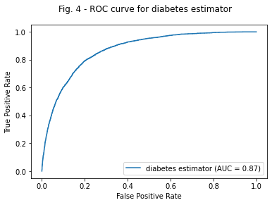
# area under the receiver operating characteristic (ROC) curve as quantifier of model quality
rocplot = metrics.RocCurveDisplay(fpr=fpr, tpr=tpr, roc_auc=roc_auc, estimator_name='diabetes estimator')

rocplot.plot()
plt.suptitle( 'Fig. 4 - ROC curve for diabetes estimator');
Feature selection
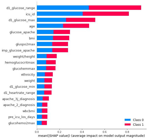
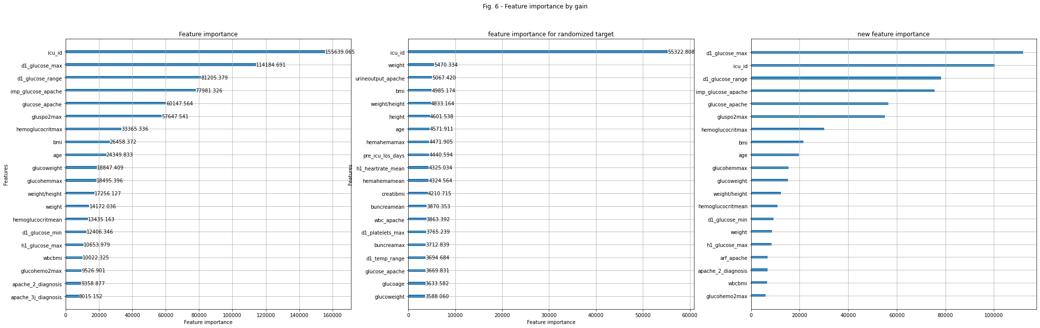
A model with fewer features will use less space and is often better understandable. For our final ensemble of models, we use model with all features and model with a selected subset of features. As a measure for feature importance we can use the shapley values., for smaller models, or feature importance function of lightgbm, for larger models with lots of trees. It can be helpful to distinguish useful features from less useful features by comparing how important features are for the real model vs how important they are for a model, where the target is randomized. Features who are also very important to fit randomized models are good at adapting to noise and their importance in the real model will be overstated. Fig. 5 shows the shapley values for the top 20 most important features on our test set. It’s a measure how much each feature contributes to the final prediction. Fig 6 shows the feature importance by gain for the gradient boosting model fitting the target and fitting the randomized target.
import shap

shap.initjs()

# shapley values to measure feature importance
shap_values = shap.TreeExplainer(bst).shap_values(X_test)

shap.summary_plot(shap_values, X_test)
bst.feature_importance('gain')
plt.suptitle( 'Fig. 5 - Feature importance from shapley values');
<Figure size 432x288 with 0 Axes>
# using shapley values to chose the best features for the model
con_cols = zip(X_train.columns,abs(shap_values[0]).mean(axis=0) )
#sorted(con_cols, key=lambda x: x[1], reverse=True)[0:400]
concols = [col for col,val in con_cols if val>0.001]
pro_cols = zip(X_train.columns,abs(shap_values[1]).mean(axis=0) )
#procols = sorted(pro_cols, key=lambda x: x[1], reverse=True)[0:400]
procols = [col for col,val in pro_cols if val>0.00]
bestcon = X_train.columns[list(set(abs(shap_values[0]).argmax(axis=1)))]
bestpro = X_train.columns[list(set(abs(shap_values[1]).argmax(axis=1)))]
take_best_features2 = set(concols).union(set(procols)).union(set(bestcon)).union(set(bestpro))
len(take_best_features2)
357
# using feature importance of the lgbm trees by looking at features that created the highest gain.
# comparing this to the best features of a model with randomized target and using those features which are
# better with the real target than with the randomized target
y_rand = np.array(y_train).copy()
np.random.shuffle(y_rand)
train_data = lgb.Dataset(X_train, label=y_rand, categorical_feature=cat_features)#, weight=w)
bst_rand = lgb.train(param, train_data, categorical_feature=cat_features)
rand_imp1 = bst_rand.feature_importance( importance_type='gain')
np.random.shuffle(y_rand)
bst_rand = lgb.train(param, train_data, categorical_feature=cat_features)
rand_imp2 = bst_rand.feature_importance( importance_type='gain')

best_feats = zip(bst.feature_importance( importance_type='gain') - (rand_imp1+rand_imp2)/2, X_train.columns)
sorted_best = sorted(best_feats, key=lambda x: x[0], reverse=True)
take_best_features = [a[1] for a in sorted_best if a[0]>0]
best_values =  [a[0] for a in sorted_best if a[0]>0]
print(X_train.shape[1], len(take_best_features))
366
# plotting the lgbm feature importance for the target, the randomized target and the difference between both.
fig, axes = plt.subplots(1,3, figsize=(35,10))
lgb.plot_importance(bst, importance_type='gain', max_num_features=20,  ax=axes[0]);
lgb.plot_importance(bst_rand, importance_type='gain', max_num_features=20,  ax=axes[1], title='feature importance for randomized target');
axes[2].barh(y=np.flipud(take_best_features[:20]), width=np.flipud(best_values[:20]), height=0.2)
axes[2].set_title('new feature importance')
axes[2].grid(True)
plt.suptitle( 'Fig. 6 - Feature importance by gain')
plt.show;


#print(len(take_best_features))
#
take_best_features = list(take_best_features)
cat_best_features = list(set(cat_features).intersection(set(take_best_features)))
# training and validating the model again with subset of selected features
train_data = lgb.Dataset(X_train[take_best_features], label=y_train, categorical_feature=cat_best_features)
bst = lgb.train(param, train_data, categorical_feature=cat_best_features)

ypred = bst.predict(X_test[take_best_features], num_iteration=bst.best_iteration)
fpr, tpr, thresholds = metrics.roc_curve(y_test, ypred)
metrics.auc(fpr, tpr) #0.86917
0.8710770006005402
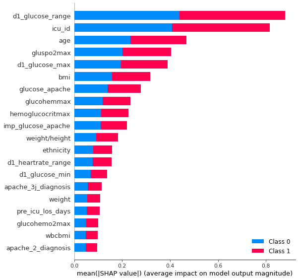
Understanding the model
It’s always useful to understand how the model is working. The shap library does a great job to show which features are important and how they influence the final prediction.
explainer = shap.TreeExplainer(bst)
shap_values = explainer.shap_values(X_test[take_best_features])

shap.summary_plot(shap_values, X_test[take_best_features])
expected_value = explainer.expected_value
if isinstance(expected_value, list):
    expected_value = expected_value[1]
print(f"Explainer expected value: {expected_value}")
Explainer expected value: -2.154676073561046
select = range(50)
features = X_test[take_best_features].iloc[select]
shap_values_sub = explainer.shap_values(features)[1]

y_pred = (shap_values_sub.sum(1) + expected_value) > 0
misclassified = y_pred != y_test.iloc[select]
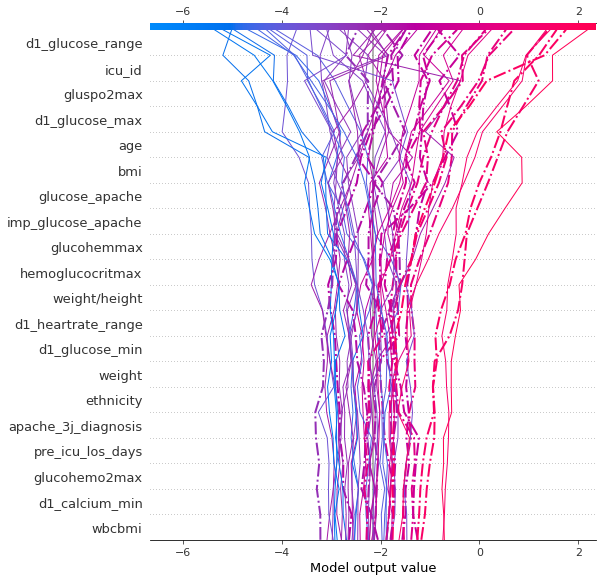
The model has a baseline of -2.1. With no features given, the patient is predicted to be non-diabetic. Fig. 7 shows how the model makes its predictions. Each feature influences the base line in a negative or positive way. The influence of the most important features is shown. Here the model gives final results between -6 and +2. When the final value is positive, the patient would be classified as diabetic. The dotted lines are misclassified cases, but of course, we could choose any cutoff we want for classification. In order to get predictive values between 0 and 1, we take the sigmoid of these values.
#shapley decision plot
shap.decision_plot(expected_value, shap_values_sub, features,  highlight=misclassified);
plt.suptitle( 'Fig. 7 - Decision  plot');
plt.show();
<Figure size 432x288 with 0 Axes>
# shapley force plot
k = np.array(select)[misclassified][3]
shap.force_plot(expected_value, shap_values_sub[k,:], X_test[take_best_features].iloc[k,:], link='logit')
Have you run `initjs()` in this notebook? If this notebook was from another user you must also trust this notebook (File -> Trust notebook). If you are viewing this notebook on github the Javascript has been stripped for security. If you are using JupyterLab this error is because a JupyterLab extension has not yet been written.
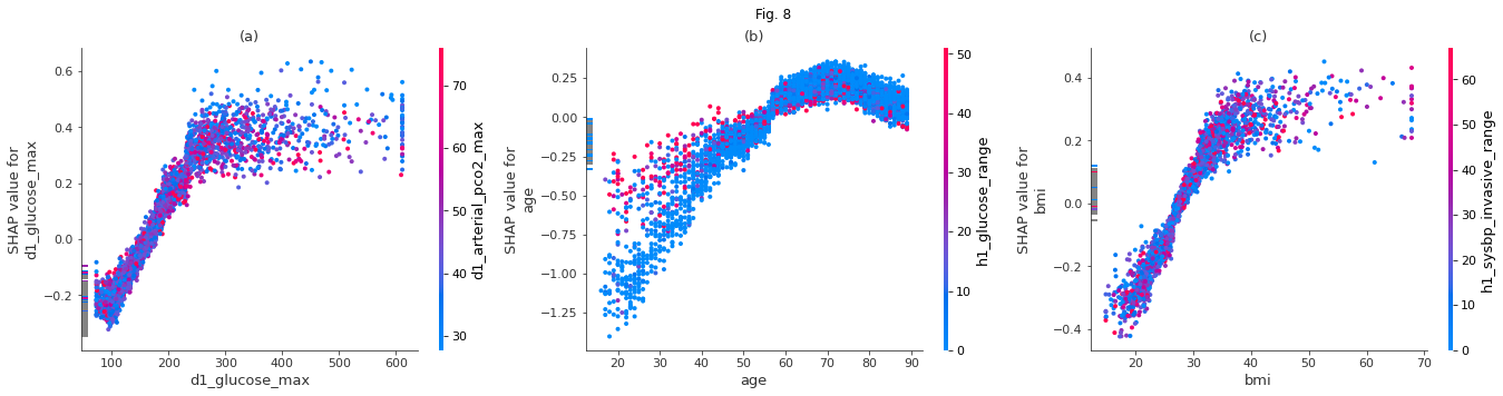
The model captures the relations between the probability of diabetes and several features in the data. In Fig. 8 (a) we can see how the prediction of diabetes depends on the maximal glucose value of the day. A glucose level above 200 increases chances of having diabetes. Fig. 8 (b) shows how the model thinks the diabetes risk changes with age. Most people with diabetes in the data seem to be above 60. The dependence on bmi in Fig 8 (c) shows an increasing risk for people with a bmi above 30. The dependence on weight (not shown here) is almost linear. However, weight correlates with age for low values. When two features correlate strongly, the plot seen by itself is less meaningful. Interaction between features can play a bigger role. The dots in the plot are colored according to a second feature for which interaction is highest.
# shapley dependence plots
fig, axes = plt.subplots(nrows=1, ncols=3, figsize=(23,5))
shap.dependence_plot("d1_glucose_max", shap_values[1], X_test[take_best_features], ax=axes[0], show=False, title='(a)')
shap.dependence_plot('age', shap_values[1], X_test[take_best_features], ax=axes[1], show=False, title='(b)')
shap.dependence_plot("bmi", shap_values[1], X_test[take_best_features], ax=axes[2], show=False, title='(c)')
fig.suptitle( 'Fig. 8')
plt.show()
Prediction and submission
For the final result we run three predictions with different seeds and slightly different values and average over them. For the competition, we have just averaged over various results along our path of testing out different things, like adding or removing features or feature imputation. The most important part when ensembling models is that they are good, but very different from each other. In the end we had an auc-score of about 0.865.
# defining hyper parameters for the final model training (chosen from previous hyper parameter testing rounds)
evals = {}
evals['lgb'] = {}
lparams = {}

seeds = [2, 3, 4]
nfold = [5, 5, 5]
lr = [0.03, 0.05, 0.01]
leaves = [77, 50, 280]
max_depth = [-1, 300, 300]
ff = [0.35, 0.22, 0.3]
ff_bynode = [0.65, 0.6, 0.5]
stratified=[False, True, True]
shuffle=[True, True, True]
n_estimators = [600, 450, 1600]
min_data_in_leaf = [20,20,240]
min_child_weight=[45, 45, 1e-3]
early_stopping_rounds = 100
verbose_eval = 0
reg_alpha = [0.7, 1, 0]
reg_lambda = [0.8, 1, 19]
verbose = -1
n_jobs = 4

for k in [0,1,2]:
    lparams[k] = dict(boosting_type='gbdt',
               objective='binary',
               metric='auc',
               learning_rate=lr[k],
               num_leaves=leaves[k],
               max_depth=max_depth[k],
               feature_fraction=ff[k],
               feature_fraction_bynode=ff_bynode[k],
               n_estimators=n_estimators[k],
               min_child_weight=min_child_weight[k],
               min_data_in_leaf=min_data_in_leaf[k],
               lambda_l1=reg_alpha[k],
               lambda_l2=reg_lambda[k],
               verbose=verbose,
               seed=seeds[0],
               n_jobs=n_jobs,)

test_preds = np.zeros(len(test_df))
dtrain = lgb.Dataset(train_df[take_best_features], y_df)
dtest = test_df[take_best_features].copy()
testlen = test_df.shape[0]
# predicting and ensembling several lgbm models, averaging over predictions for each fold and averaging over ranked prediction for each model
for i, seed in enumerate(seeds):
    print(f'Training Model with SEED : {seed}')
    evals['lgb'][i] = lgb.cv(lparams[i],
                             dtrain,
                             nfold=nfold[i],
                             stratified=stratified[i],
                             shuffle=shuffle[i],
                             num_boost_round=n_estimators,
                             early_stopping_rounds=early_stopping_rounds,
                             verbose_eval=verbose_eval,
                             return_cvbooster=True,
                             seed = seed,
                             show_stdv=True)
    print(f'SEED {i} Average fold  AUC {np.round(max(evals["lgb"][i]["auc-mean"]),5)}')
    test_preds += stats.rankdata(np.mean(evals['lgb'][i]['cvbooster'].predict(dtest, num_iteration=evals['lgb'][i]['cvbooster'].best_iteration), axis=0)) / (testlen * len(seeds))
Training Model with SEED : 2
SEED 0 Average fold  AUC 0.87231
Training Model with SEED : 3
SEED 1 Average fold  AUC 0.87087
Training Model with SEED : 4
SEED 2 Average fold  AUC 0.87205
submission = pd.DataFrame.from_dict({
    'encounter_id':test_id,
    'diabetes_mellitus':test_preds,
})
submission.to_csv('submission.csv', index=False)